Gladiators, ready! Pricing models fight it out
Nonplussed by neural networks? Intimidated by the jargon? You can’t afford to
be, not in the fast-paced pricing arena. Four actuaries put two cutting-edge
models to the test, to see which wins out.
In the competitive world of pricing, actuaries are racing to deliver greater accuracy in
smaller timeframes – and a host of new and increasingly sophisticated modelling
architectures can be used to gain that elusive edge.
Here, we describe and test two of these modelling technologies, the combined
actuarial neural network and the LocalGLMnet, which use classical statistical
methods alongside neural networks to improve predictive accuracy. Every second
and penny counts; used wisely, these solutions may present an advantage.
Putting it simply
Neural networks can seem intimidating, with the terminology around these models
no doubt contributing to this. The jargon, with its neurons, activation functions and
layers, can sound foreboding at first – but don’t let it scare you off. Let’s demystify
the nuts and bolts of neural network architecture.
To draw from common actuarial and statistical knowledge, we can think of a neuron
as a univariate binomial generalised linear model (GLM). In this simple case, the
activation function is the logistic function. If we were building a GLM, we would be
nearly finished, but a neural network consists of several such GLMs working
together. How? Each neuron calculates a single number, and a collection of these
form a layer. There are two mandatory layers (the input and output); any layers in
between are referred to as hidden layers. The number of neurons in a layer, and the
number of layers in the neural network, can be set manually or through a tuning
process.
The first (input) layer consists of our predictors, which are then passed to neurons in
the first hidden layer. Inside each neuron, the inputs are scaled and shifted by
weights and biases before feeding through the activation function. After these
calculations we obtain an output of the first hidden layer, which is then passed to the
second layer, and so on, until we reach the network’s output layer. When information
flows in this forward direction, from input layers to output layers, the model is known
as a feedforward neural network (FFNN).
Why do we say neural networks are trained, or learn? As a comparison, when fitting
a linear regression model, numerical techniques are used to converge on a solution to a closed-form problem. In neural networks, however, there are so many model parameters and so many intractable interactions between them that such closed-form formula does not exist. We use iterative optimisation techniques to tweak randomly initiated parameters until they produce an output close to the given target
variable.
Combined actuarial neural networks
A combined actuarial neural network (CANN) embeds a GLM into a neural network
using a skip connection that directly links the input layer to the output layer (Figure
1).
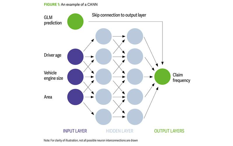
It is essentially a neural network that uses the benchmark GLM’s predictions while
learning additional interactions among variables to improve the overall model’s
predictive power. There are three common approaches to using a CANN:
- The GLM element is non-trainable, so the benchmark GLM is always
present and only the network part changes. This is the form of CANN included
in the analysis to follow. - The entire network parameter can be trained, meaning the benchmark
GLM can be modified. - A trainable credibility weighting can be introduced for the fixed GLM
element within the CANN.
While CANN may not generally outperform pure neural networks in minimising the
objective loss function, its value for pricing teams lies in uncovering nuanced
interactions that can enhance existing GLMs in production.
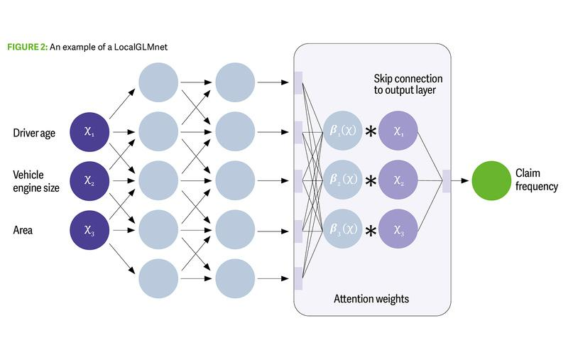
LocalGLMnet
This structure predicts GLM’s coefficients for each individual record using a neural
network, leveraging the GLM’s advantages in terms of explainability. However, it
gains predictive accuracy by allowing the coefficients to vary for each record. The
LocalGLMnet uses a skip connection (different from that used in the CANN), directly
linking the input features to the output layer. This provides a linear term in the model,
which bypasses the neural network, and then weights these terms with potentially
non-linear weights.
Successfully training this neural network leaves us with a highly predictive model and
a set of beta coefficients (attention weights) for each observation (Figure 2). Now we
can interpret the prediction in a familiar way but also analyse the attention weights
and how they vary for different predictors.
Results
Now that we have conceptually described these two new models, let’s road-test
them and see how they perform on real-world data. In this case, we use them to
predict the frequency of third-party motor liability claims for individual customers,
using a publicly available dataset with 680,000 records and 11 features relating to
motor policies of a French insurer. This dataset is commonly used in literature on
actuarial models and model benchmarking.
We studied CANN and LocalGLMnet and included the GLM and FFNN models for
comparison. A simple intercept model is also included for reference. A full
description of the implemented models is beyond the scope of this article, so we will
focus on high-level results and conclusions from the exercise. A more detailed
presentation of this work will be available in an accompanying blog post on Towards
Data Science and a GitHub repository (github.com/Karol-
Gawlowski/ADSWP_NN ).
Every second and every penny counts; used wisely, these solutions may present an advantage
Table 1 shows the results of a cross-validation (CV) exercise over five folds of the
data. In a five-fold CV exercise, the model is fitted once over four partitions of the
modelling data, then tested on the fifth unseen partition. This is done five times, with
a different unseen partition of data tested each time. The metric used to assess
model performance here is the total Poisson deviance, where a lower deviance on
the unseen partition is preferred. The ‘pinball score’ of the best neural net model,
and of the GLM, is also shown for each partition. This score is essentially the
percentage reduction in deviance from a null model to the model of interest.
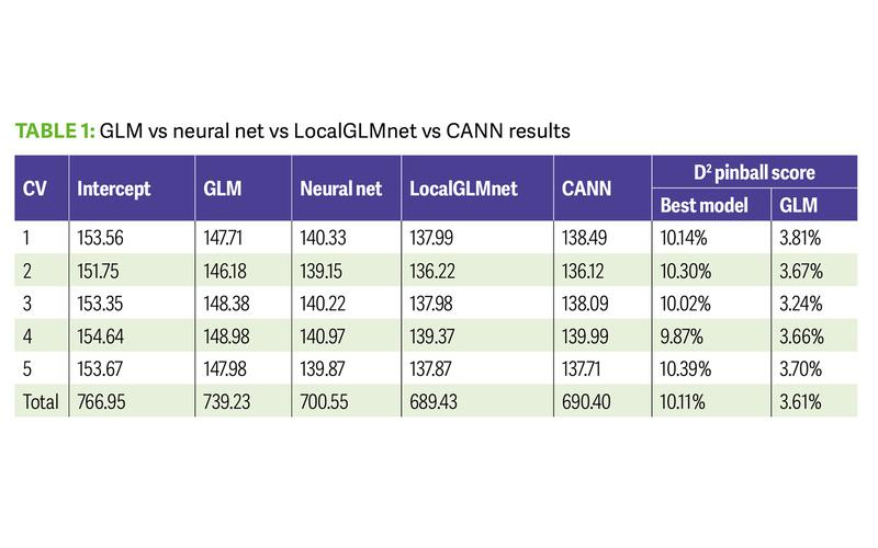
We can see that the total Poisson deviance of CANN and LocalGLMnet are about
the same, and are winning the race in terms of that metric. They are followed up by
the FFNN, with the GLM coming in last. Most notably, the pinball score of the neural
nets is approximately three times better than that of the GLM, over each unseen
partition.
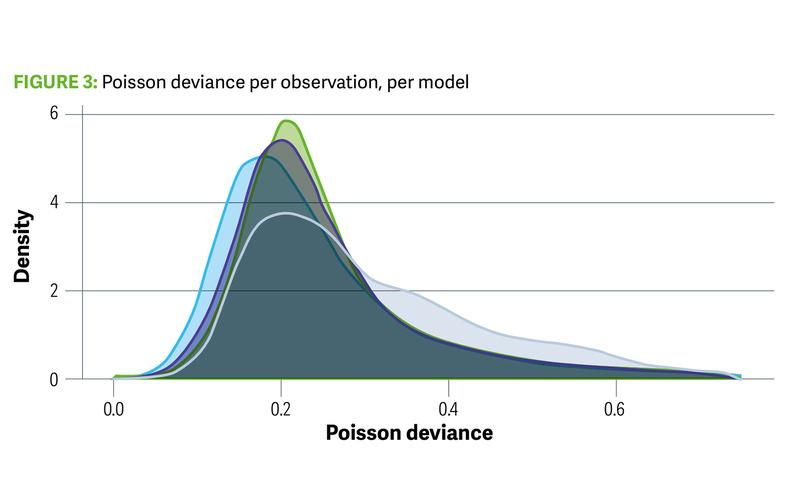
We have looked at the total Poisson deviance, but we can look at the full distribution
of values for each model as well. This is shown in the Figure 3, where we can see
that the GLM model has its weight of deviances further from 0 when compared with
the net models (CANN, FFNN, LocalGLMnet). LocalGLMnet appears to do best by
this measure.
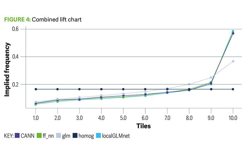
Using a lift chart, we can assess how well these model architectures distinguish
between high and low-risk policies. Figure 4 separates policies along the x axis in
deciles, according to how risky the respective models view those policies. For
example, the first decile contains the policies whose GLM prediction is in the lowest
10% of policies for that model. The first decile also contains the policies whose
prediction of frequency is in the lowest 10% for each of the FFNN, CANN and
LocalGLMnet models. Then, for each model’s lowest decile of policies, we calculate
the actual average observed frequency and plot this point. This is calculated and
plotted for all 10 deciles. The model that is best at distinguishing between low and
high risk policies will then have the greatest lift between the low and high deciles in
the chart. In Figure 4 we can see that neural network models are more successful at
this task than a GLM.
What does it mean for pricing?
It appears these newer architectures have more predictive power than legacy
models. As other studies have found, sacrifices are made in terms of transparency
and explainability when departing from GLM architecture, so explainable artificial
intelligence (XAI) may be required to help with model interpretation. However,
LocalGLMnet makes progress in this area where a local GLM structure is retained.
The CANN could also be a useful concept for insurers that have already developed a
GLM, as the neural network that is combined with the GLM may reveal opportunities
for further model refinement.
We should note that the results and conclusions here are somewhat specific to the
dataset used and the particular implementation of the models. If the GLM model
were optimised further, it is possible that we could observe different results.
The new technologies covered in this study may present a distinct edge in the
competitive world of insurance pricing. However, the care and skill of forward-
thinking and dynamic pricing teams will be required to steer these technologies
towards a podium finish.
The IFoA Actuarial Data Science Working Party would like to credit for their
original development and research on these architectures: Mario V Wüthrich,
Michael Merz and Jürg Schelldorfer for CANN; Ronald Richman and Mario V
Wüthrich for LocalGLMnet.
Karol Gawlowski is a predictive modeller at Allianz Commercial and chair of the
IFoA Actuarial Data Science Working Party
John Condon is a lecturer in actuarial science, School of Mathematical Sciences,
University College Cork
Jack Harrington is a senior pricing actuary at AXA Insurance
Davide Ruffini is a pricing actuary at AmTrust Assicurazioni in Milan
Image credit: Shutterstock
Enjoyed this read?
This article was originally published in The Actuary, March 2024 issue
https://www.theactuary.com/2024/03/05/gladiators-ready-pricing-models-fight-it-out
Head over theactuary.com for more insightful content.